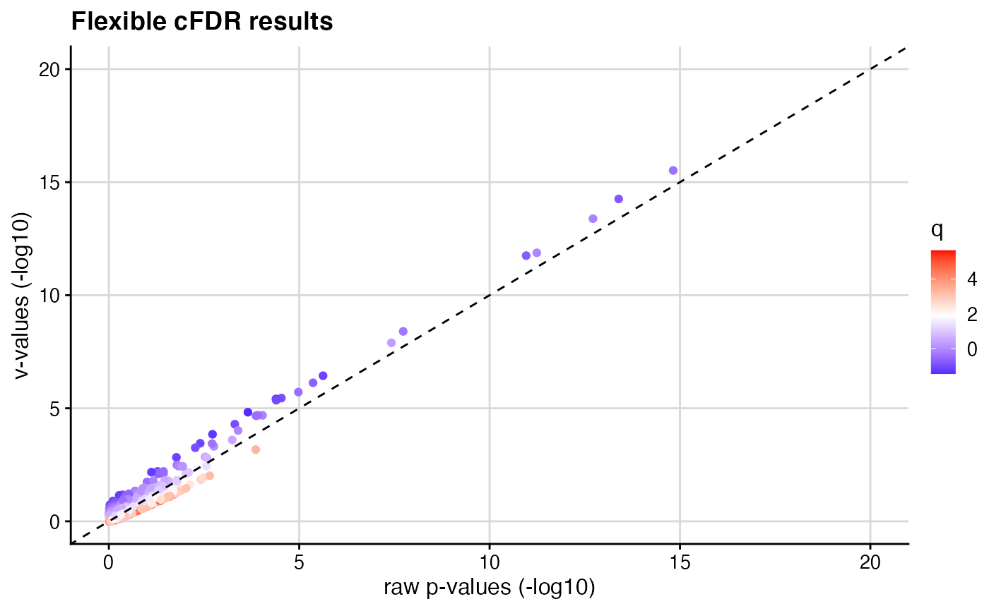
Plot -log10(p) against -log10(v) and colour by q

log10pv_plot(p, q, v, axis_lim = c(0, 20))

Arguments

p	p values for principal trait (vector of length n)
q	auxiliary data values (vector of length n)
v	v values from cFDR
axis_lim	Optional axis limits

Value

ggplot object

Details

Can be used to visualise the results from Flexible cFDR

Examples

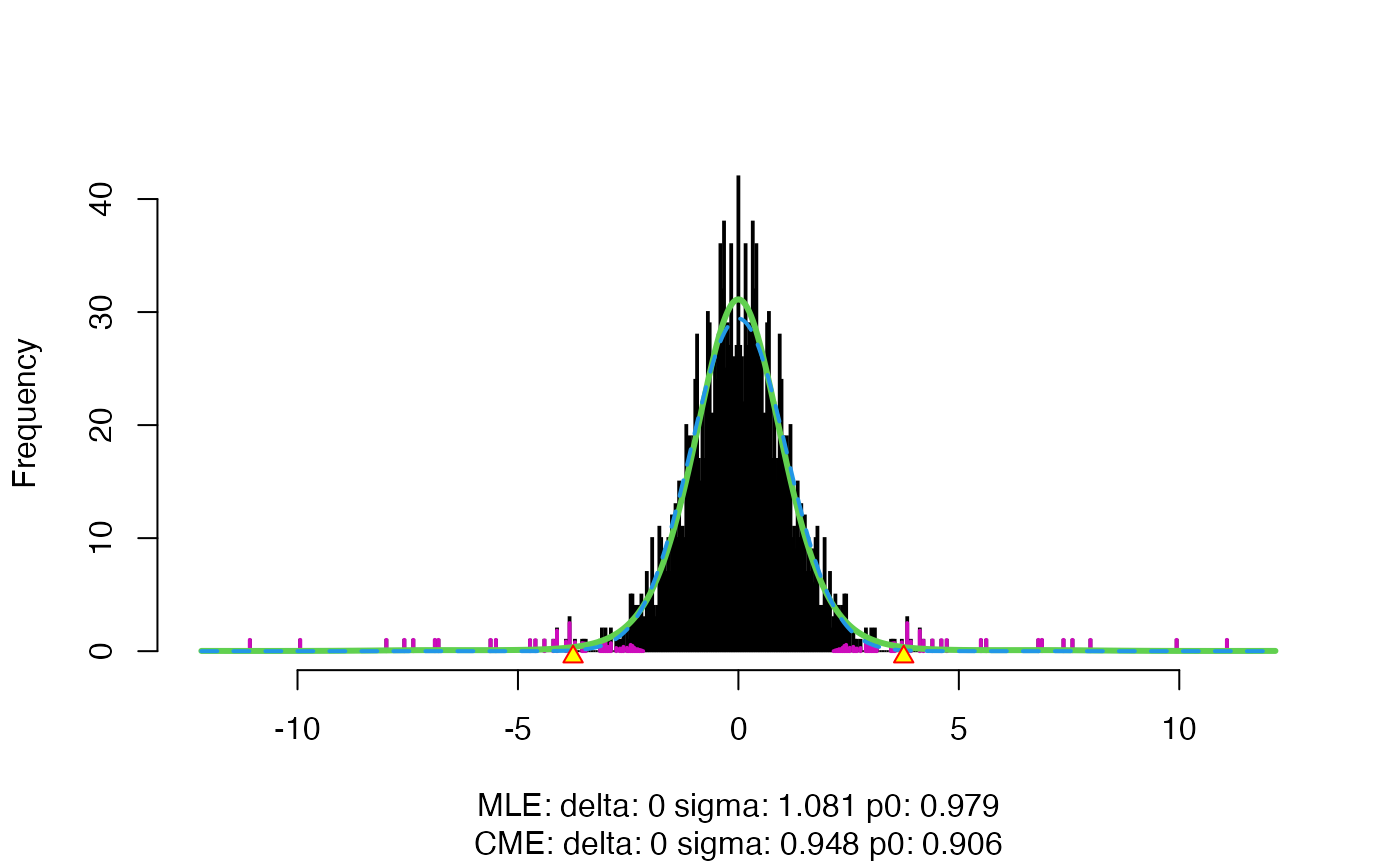
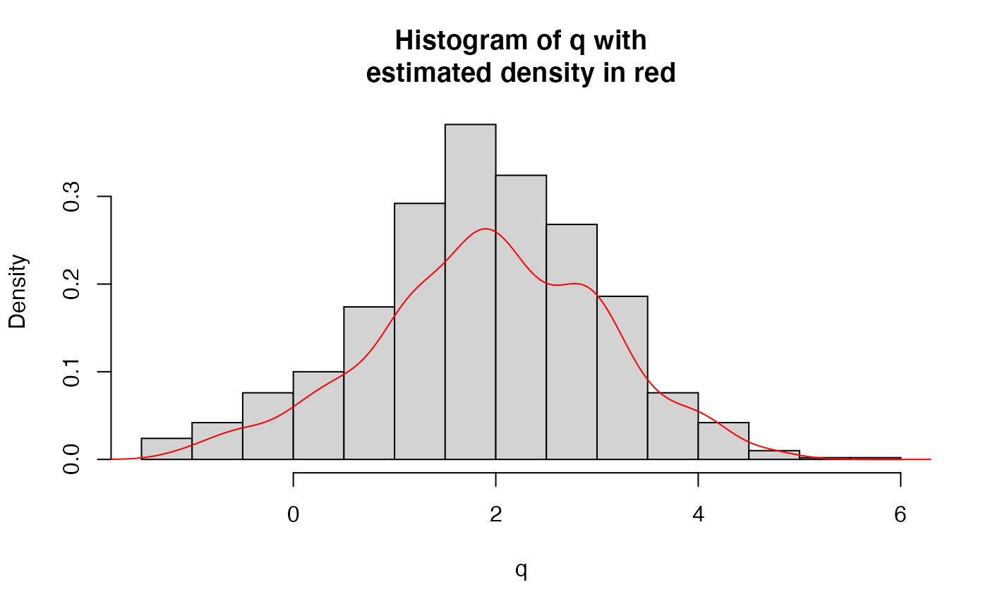
# \donttest{
# this is a long running example

# In this example, we generate some p-values (representing GWAS p-values)
# and some arbitrary auxiliary data values (e.g. representing functional genomic data).
# We use the flexible_cfdr() function to generate v-values and then the log10pv_plot() function
# to visualise the results.

# generate p
set.seed(1)
n <- 1000
n1p <- 50 
zp <- c(rnorm(n1p, sd=5), rnorm(n-n1p, sd=1))
p <- 2*pnorm(-abs(zp))

# generate q
mixture_comp1 <- function(x) rnorm(x, mean = -0.5, sd = 0.5)
mixture_comp2 <- function(x) rnorm(x, mean = 2, sd = 1)
q <- c(mixture_comp1(n1p), mixture_comp2(n-n1p))

n_indep <- n

res <- flexible_cfdr(p, q, indep_index = 1:n_indep)

log10pv_plot(p = res[[1]]$p, q = res[[1]]$q, v = res[[1]]$v)
# }