Introductory vignette • fcfdr

The fcfdr R package implements the cFDR framework and is applicable for a wide variety of auxiliary covariates. This is in contrast to earlier empirical cFDR methods (Liley and Wallace 2021; https://github.com/jamesliley/cfdr) that only support auxiliary \(p\)-values from related traits. A direct utility of fcfdr is to leverage relevant functional genomic data with GWAS \(p\)-values to increase power for GWAS discovery. The method generates “\(v\)-values” which can be interpreted as GWAS \(p\)-values that have been re-weighted according to the auxiliary data values. Since the \(v\)-values are analogous to \(p\)-values, they can be used directly in any error-rate controlling procedure.

The fcfdr R package contains two key functions:

flexible_cfdr: Implements cFDR leveraging \(\textbf{continuous}\) auxiliary covariates.
binary_cfdr: Implements cFDR leveraging \(\textbf{binary}\) auxiliary covariates.

Both functions require two parameters to be specified:

p: GWAS \(p\)-values for the trait of interest (vector of per-SNP \(p\)-values)
q: Auxiliary data values (vector of per-SNP auxiliary data values).

The flexible_cfdr function also requires the indices of an independent subset of SNPs (indep_index parameter; see LDAK vignette) whilst the binary_cfdr function requires group indices for each SNP (group parameter; typically the chromosome or LD block index for each SNP).

For further details, including instructions to generate indep_index, examples of auxiliary data to leverage and instructions to apply cFDR iteratively, please see the Extra Information vignette.

Simple walk-through example

Firstly, load the Flexible cFDR R package:

library(fcfdr)

Next, simulate \(p\)-values for 50,000 genetic variants, including 500 associated variants.

set.seed(1)
n = 50000
n1p = 500 # associated variants
zp = c(rnorm(n1p, sd=5), rnorm(n-n1p, sd=1)) # z-scores
p = 2*pnorm(-abs(zp)) # convert to p-values
hist(p)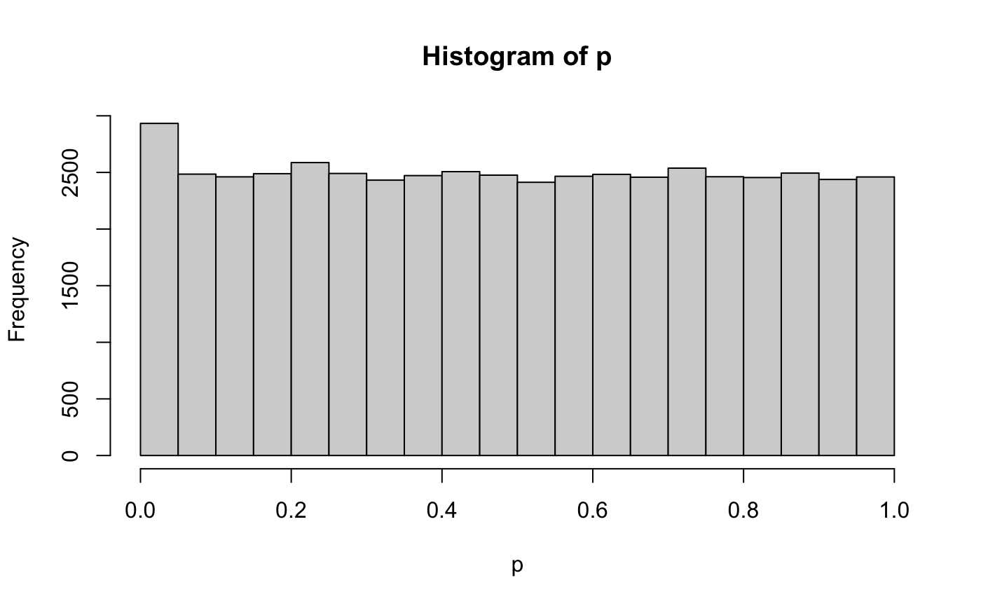

We simulate relevant auxiliary data from a mixture normal distribution (\(q\)). The associated SNPs (with indices 1-500) are sampled from \(N(-0.5, 0.5^2)\) and the non-associated SNPs (with indices 500-50000) are sampled from \(N(2,1)\).

mixture_comp1 <- function(x) rnorm(x, mean = -0.5, sd = 0.5)
mixture_comp2 <- function(x) rnorm(x, mean = 2, sd = 1)
n = length(p)
z = runif(n)

q <- c(mixture_comp1(n1p), mixture_comp2(n-n1p))
hist(q)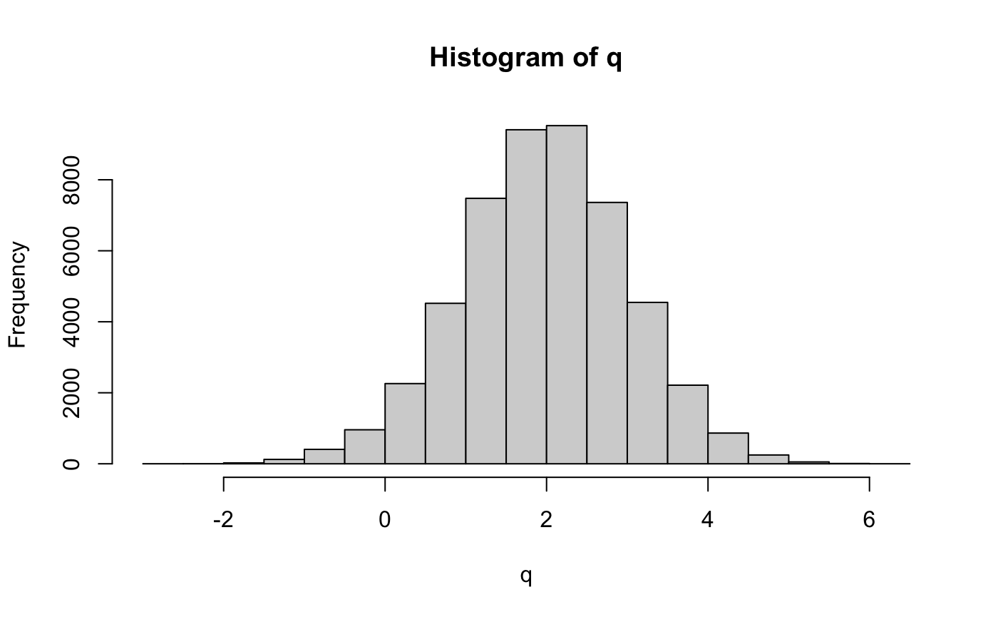

We can use the corr_plot function to visualise the relationship between \(p\) and \(q\). We observe that low \(p\)-values (i.e. high \(-log10(p)\)) are enriched for low \(q\) values.

corr_plot(p, q)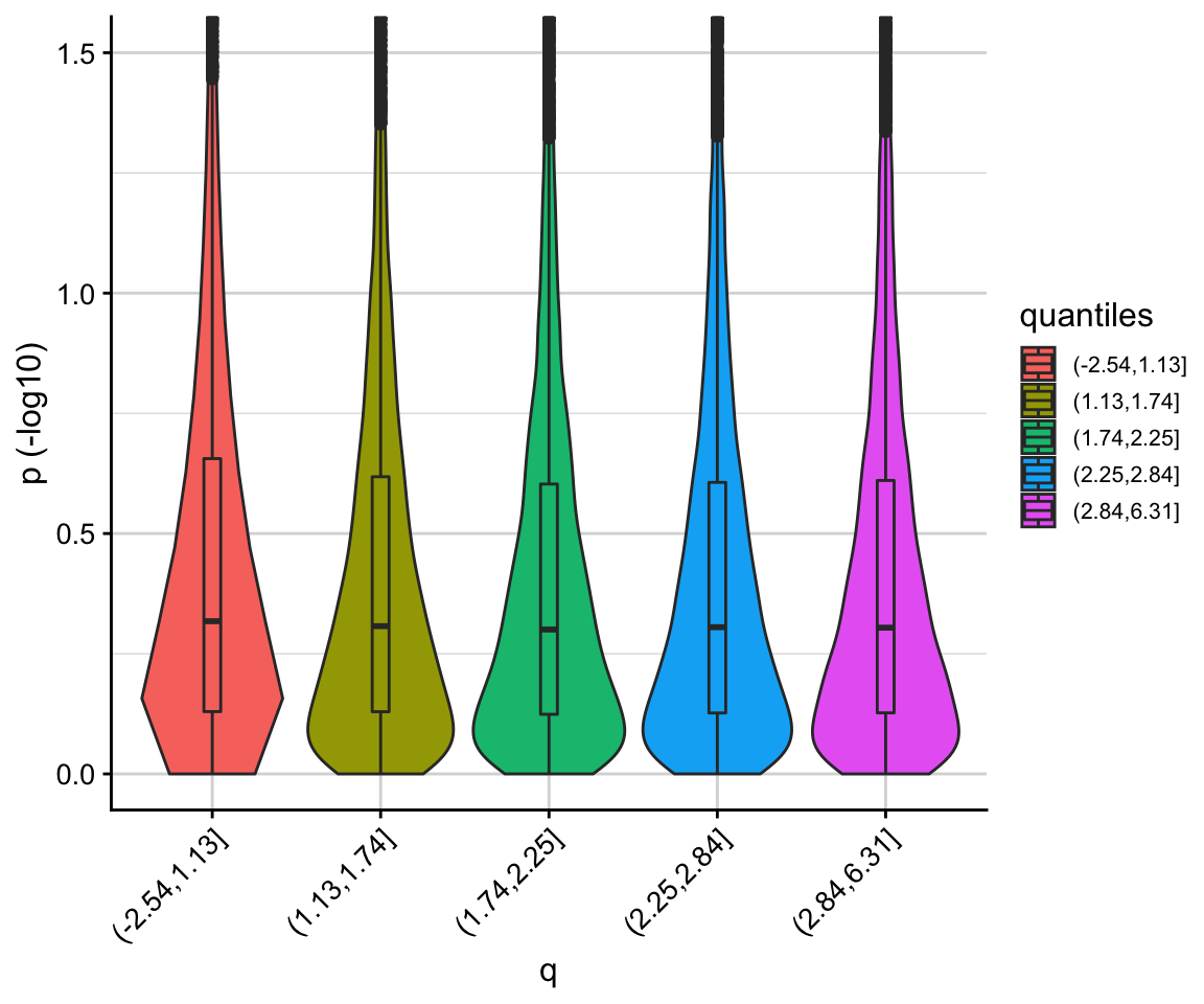

This is also clear from the stratified QQ plot.

stratified_qqplot(data_frame = data.frame(p, q), prin_value_label = "p", cond_value_label = "q", thresholds = quantile(q)[-1])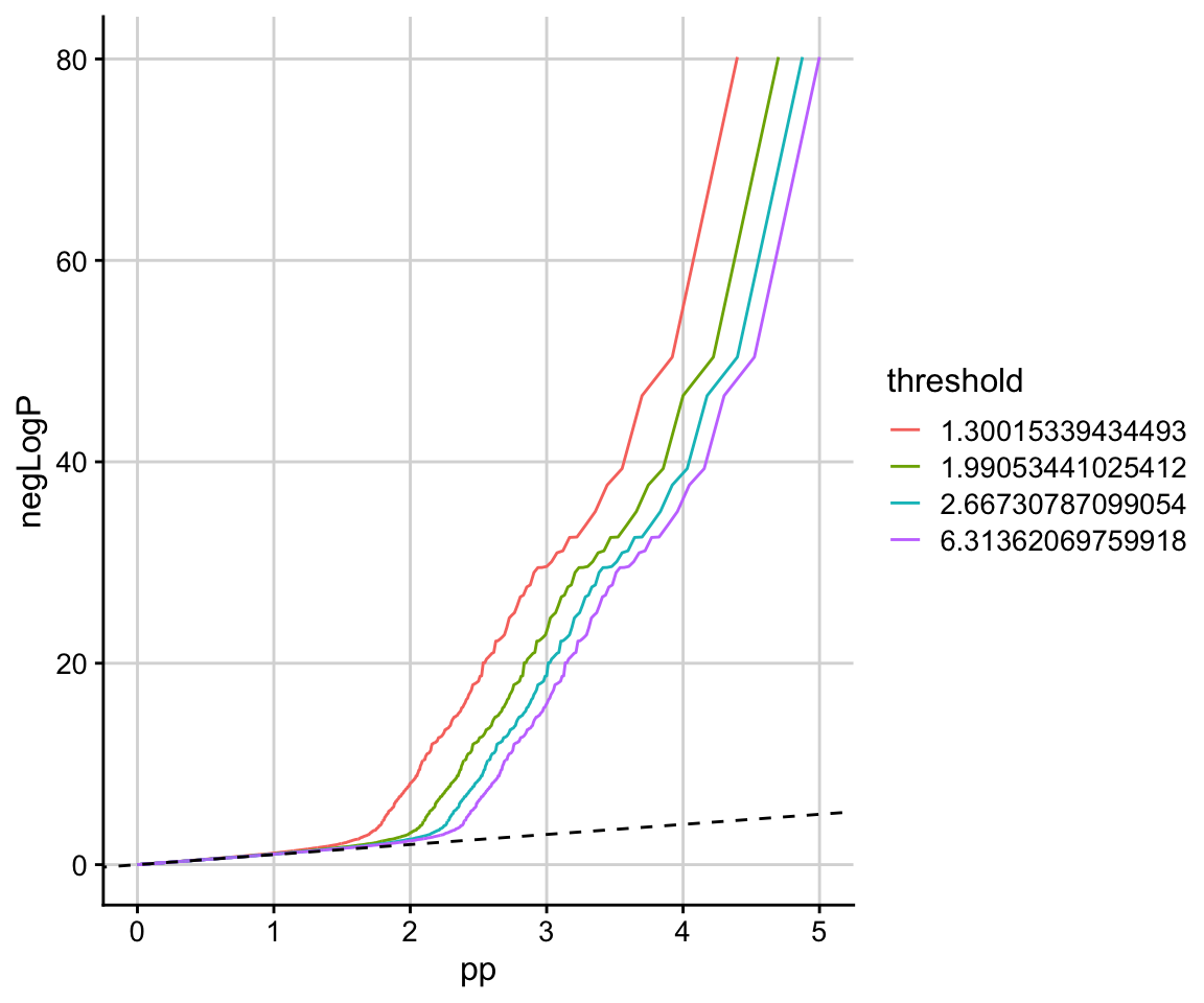

We are now ready to use the flexible_cfdr function to derive the \(v\)-values. Note that for the purpose of the vignette, we do not specify an independent subset of SNPs, however for real analyses this parameter should be specified appropriately to avoid biased bandwidth estimations when fitting the KDE. Subsets of independent SNPs can be readily found using PLINK or LDAK - see the vignette for deriving LDAK weights here.

By default, flexible_cfdr prints some useful plots so that users can evaluate the accuracy of the KDE that is estimated in the method.

(This line of code will take approximately 4 minutes to run.)

res <- flexible_cfdr(p, q, indep_index = seq(1, n, 1))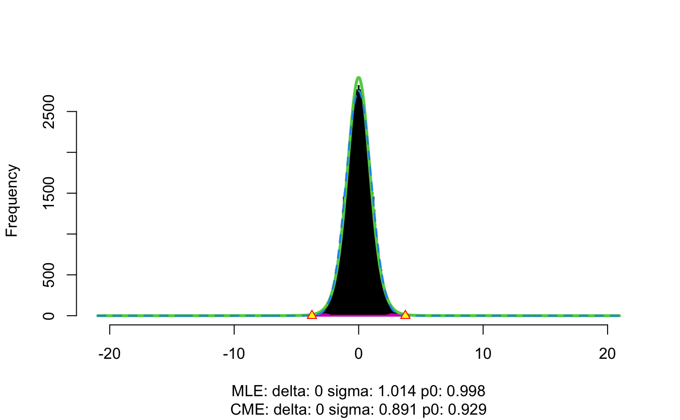

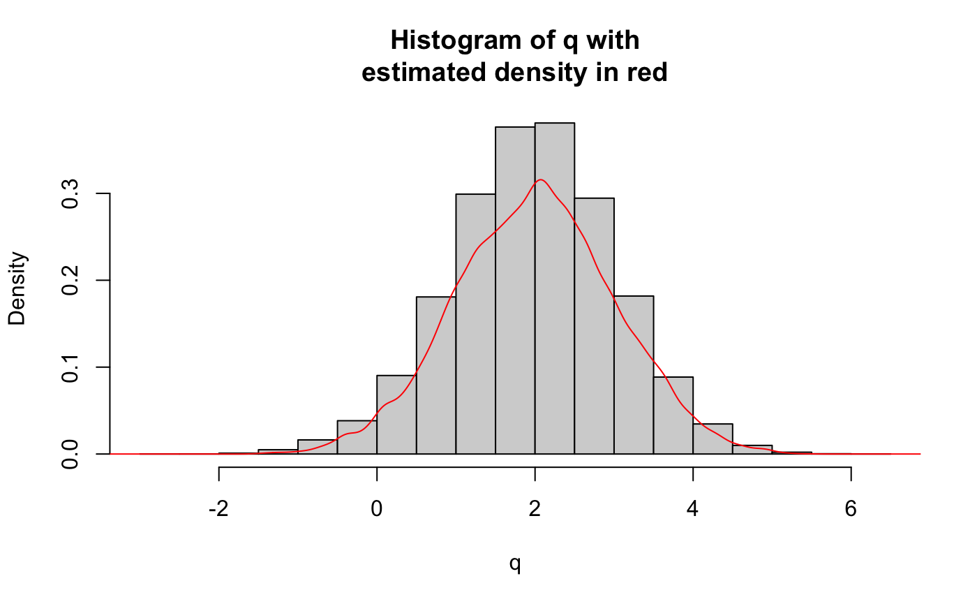
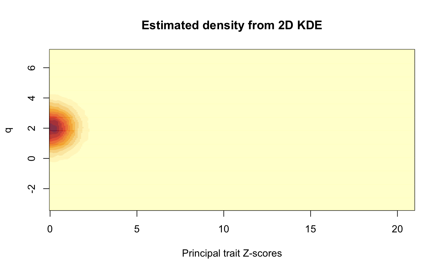
The output from the function is a list of length two. The first element is a data.frame containing the \(p\)-values (input parameter p), the auxiliary data values (input parameter q) and the generated \(v\)-values. The second element contains auxiliary data, such as how many data-points were left-censored in the method and/or spline corrected. In this example, we can see that a value of \(q=-0.169\) was used for left censoring (any auxiliary data values smaller than this were set to this value) which results in 1108/50000 (2% of) data points being left censored. We also see that 109 (0.2% of) data points were spline corrected.

str(res)
#> List of 2
#>  $ :'data.frame':    50000 obs. of  3 variables:
#>   ..$ p: num [1:50000] 1.73e-03 3.59e-01 2.94e-05 1.51e-15 9.94e-02 ...
#>   ..$ q: num [1:50000] -0.325 -0.297 -0.458 -0.383 -0.578 ...
#>   ..$ v: num [1:50000] 2.07e-04 4.94e-02 3.48e-06 1.70e-16 1.22e-02 ...
#>  $ :'data.frame':    1 obs. of  3 variables:
#>   ..$ q_low     : num -0.169
#>   ..$ left_cens : int 1108
#>   ..$ splinecorr: int 109

p = res[[1]]$p
q = res[[1]]$q
v = res[[1]]$v

Note that the cFDR framework requires that low \(p\)-values are enriched for low \(q\) values, so that if the correlation between \(p\) and \(q\) is negative then the function intrinsically flips the sign of \(q\), meaning that the \(q\) values reported in the data.frame output may be \(q:=-q\).

We can then visualise the results using the pv_plot and log10pv_plot functions.

We observe that \(v\)-values for SNPs with high \(q\) values are increased, whilst those for SNPs with low \(q\) values are decreased.

pv_plot(p = p, q = q, v = v)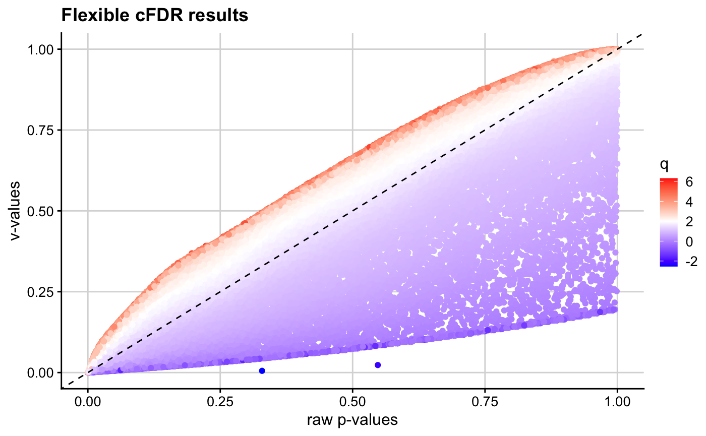

log10pv_plot(p = p, q = q, v = v, 
             axis_lim = c(0, 10)) # zoom in to interesting region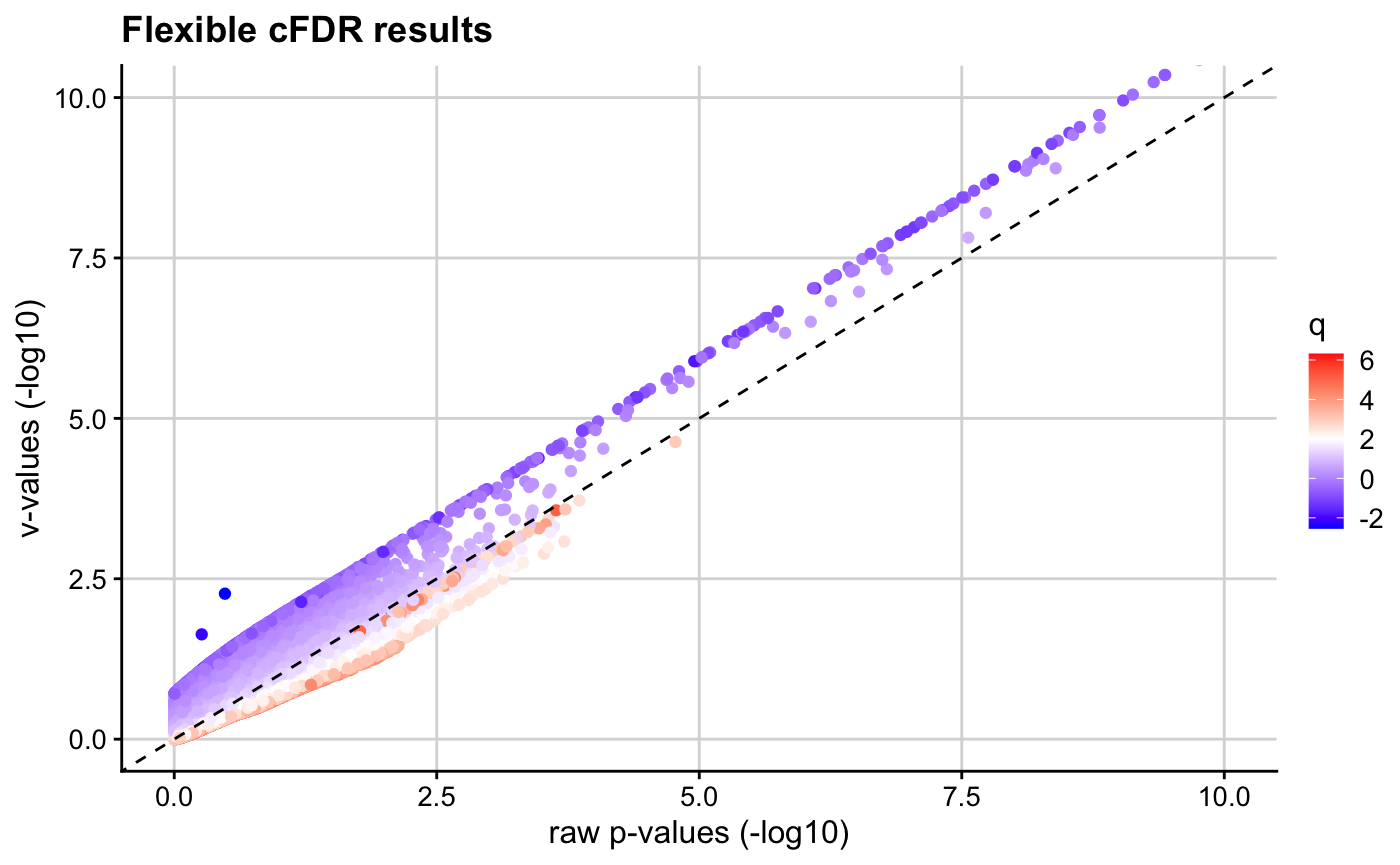

Finally, we run the Benjamini-Hochberg procedure on the \(v\)-values and control the FDR at 0.05. This means that we are willing to accept up to 5% of the associations to be false positives.

hit = which(p.adjust(v, method = "BH") <= 0.05)

For comparison, we do the same to the raw p-values:

hit_p = which(p.adjust(p, method = "BH") <= 0.05)

‘True’ associations are those with indices 1-500, so the proportions of false discoveries are

# cFDR
1 - (length(intersect(hit,c(1:500)))/length(hit)) 
#> [1] 0.04363636

# p-value
1 - (length(intersect(hit_p,c(1:500)))/length(hit_p))
#> [1] 0.02262443

Altogether, the cFDR method has found 47 new associations that are true whilst controlling the FDR.

# number of extra true associations identified by flexible cFDR
length(which(hit[!hit %in% hit_p] <= 500))
#> [1] 47